Microbial De Novo Genome Assembly from Short-Read Data

This is yet another tutorial on microbial genome assembly. This is actually the Part 2 of tutorial series: NGS Workflow for Genome Assembly to Annotation for Hybrid Bacterial Data 

In this series we’ll be use hybrid sequencing data (Illumina and Nanopore). This tutorial has five parts. 

Part 1: Downloading and preparing data

Part 2: Assembly with short-reads.

Part 3: Assembly with long-reads.

Part 4: Hybrid assembly (long- and short-reads).

Part 5: Bacterial genome annotation with Bakta and Beav.

Disclaimer: This post is a work in progress. This is genome assembly and annotation workflow that I use for microbial genomics. Previously, I used this template to teach different class in OSU as well as in other training facilities.

---

SPAdes is a very good de novo bacterial sequence assembly program. For bacterial genome assembly, it is THE program to rule them all (for short-reads)! It’s a k-mer graphed based tool, that means it generates a graph based on kmers, and from the graph, it create the assembly. Therefore, it’s very good, but it is so resource-hungy (takes lot of RAM), and time-consuming. However, there are some other tools based on SPAdes like Shovill which run faster.

Software Installation

Don’t forget to peruse the user manual for each tools!

conda install bioconda::bbmap
conda install bioconda::fastqc
conda install bioconda::fastp
conda install bioconda::spades
conda install bioconda::bandage

Getting the data-set

Anyway, we need to check the quality of the Illumina reads first. If you have your own raw-data, you can use that. You can also download some publicly available bacterial genome as mentioned in this post.

If you are just trying to test out the tools without taking long time to run them, you can resample the reads of your fastq files using reformat.sh from bbmap. The following commands will randomly sample 10% reads from both of your fastq files (forward and reverse):

reformat.sh in1=strain1_R1.fq.gz in2=strain1_R2.fq.gz out1=strain1_sampled_R1.fq.gz out2=strain1_sampled_R2.fq.gz samplerate=0.1

Tools and installation

All softwares, if not mentioned, can be found in bioconda and installable by conda.

Determining taxonomy

After getting the raw data, a tool called sendsketch.sh from bbtools is super handy to quickly check taxonomy from the raw fastq files (and the assembled-contigs). It creates a kmer-based hash fingerprints, and compare that with reference databases (and extremely fast)!

K-mer sketches are a compact representation of the sequence data and are used for fast comparison and identification.The following script loops through each raw FASTQ file, generates a k-mer sketch using the sendsketch.sh tool, and saves the sketch files. This step is important for identifying and characterizing the samples based on their k-mer profiles.

#!/bin/bash
#unset PYTHONPATH

for infile in `ls -1 ./raw/*.fastq.gz`; do
        dataset=`basename "$infile" | sed 's/.fastq.gz//g'`
        echo -e "$infile $dataset"
        sendsketch.sh -da in=$infile out=./sketches/${dataset}.sketch
done

Once the .sketch files have been generated, we can summarize those using the following script. This is a fast way to characterize the barcoded samples with good confidence.

To extract relevant information from the generated sketch files and summarize it in a tabular format. This provides a quick overview of the samples’ genome size, average nucleotide identity (ANI), and taxonomic classification.

The script creates a summary file with columns for strain ID, ANI, genome size, and taxonomic name. It extracts these values from the sketch files and appends them to the summary file. This allows for easy comparison and interpretation of the k-mer sketch results.

#!/bin/bash

# Create the header for summary file
echo 'strainID  ANI     gSize   taxName' > sketch_summary.tsv

# Loop through sketch report and extract necessary column from the first hit
for sketch in `ls -d *.sketch`;
do
        strainid=`basename "$sketch" | sed 's/.sketch//g'`
        ani=`tail -n +4 $sketch | head -n 1 | cut -f 3`
        gSize=`tail -n +4 $sketch | head -n 1 | cut -f 10`
        taxa=`tail -n +4 $sketch | head -n 1 | cut -f 12`
        echo "${strainid}       ${ani}  ${gSize}        ${taxa}" >> sketch_summary.tsv
done

Quality-Assessment of FastQ

Normally, we want to visualize the quality of the raw-reads before we start. For that, we can use FastQC:

fastqc strain1_R1.fastq.gz
fastqc strain1_R2.fastq.gz

Or, using bash wildcard:

fastqc *fastq.gz

FastQC produces html report of the raw-reads. It’s a good idea to process the raw reads further, and remove any adapter sequences. For example, we can use another program names FastP to pre-process the reads further for assembly. We can remove any reads which has overall quality below some threshold:

fastp -i strain1_R1.fastq.gz -I strain1_R1.fastq.gz -o strain1_R1.fastp.fastq.gz -O strain1_R2.fastp.fastq.gz -e 28

Notice, the fastp outputs has fastp.fastq.gz suffix.

The -e option defines average quality, i.e. if one read’s average quality is below some threshold, it would be dropped.

Now, we can repeat FastQC again:

fastqc *fastp.fastq.gz

Once we are happy with the quality of the reads, we can move to assembly!

Sequence Assembly

Normally, we would run the following:

spades.py -o output_directory --phred-offset 33 --careful -1 strain1_R1.fastp.fastq.gz -2 strain1_R2.fastp.fastq.gz -k 21,33,55,77,99 

But if we have limited resources, we can specify the run with fewer ram, fewer k-mer estimation, etc:

spades.py -o output_directory --phred-offset 33 -1 strain1_R1.fastp.fastq.gz -2 strain1_R2.fastp.fastq.gz -k 21,33,55 -t 4 -m 10 --only-assembler

Here, the options of the SPAdes are following:

-o Output folder, -t # Threads, -m Memory in Gigabytes –only-assembler no error correction -k list of k-mer sizes (must be odd and less than 128).

The SPAdes annotation outputs are written in the defined output_directory. There are two main files that we need later: contigs.fasta which contains all the assembled contigs, and assembly_graph.fastg, which contains the graph data that we can visualize.

Getting assembly statistics

There are multiple tools for doing that. A quick and dirty approach is to use an old perl program called assemblathon. You can download it and it’s dependency in your working directory by:

wget https://raw.githubusercontent.com/KorfLab/Assemblathon/refs/heads/master/assemblathon_stats.pl

wget https://raw.githubusercontent.com/ucdavis-bioinformatics/assemblathon2-analysis/refs/heads/master/FAlite.pm

Now run assemblathon:

perl assemblathon_stats.pl spades/output_directory/contigs.fasta

Quast is also good tool, specially if there are any particular reference you want to compare the assembly with. Also it is handy when you already have annotation from current assembly. So, we will introduce Quast later.

Visualizing assembly graph

Last but not the least, we can visualize the assembly graph by using a tool called Bandage, and it takes assembly_graph.fastg file as input:

bandage image assembly_graph.fastg output.png

For example, the assembly from the 1% resampled Agrobacterium reads look like the following (which are essentially bunch of very short contigs):

If you run the assembly without resampling for Shigella, i.e. complete raw data, the assembly will look like this:

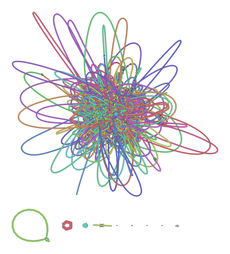
Notice, it looks like a giant hair-ball! That’s because the it’s very hard for the assembler to resolve the contigs, thats why the graph is connecting the repeating sequences.

Are there any contaminants?

We can again use the `sendsketch.sh` to check the assembled contigs individually, and look for any potential contamination. However, we will be using the mode=sequence to search the each contigs individually, and determine its taxonomy:

sendsketch.sh mode=sequence in=spades/output_directory/contigs.fasta out=sketches/contigs.sketch

Check the `contigs.sketch` file to look for any obvious contamination!

Now go to Part 3 of tutorial series: NGS Workflow for Genome Assembly to Annotation for Hybrid Bacterial Data