

This is the Chapter 10 of Py4Bio.
Personally, I’m not a big fan of Matplotlib. There are many great plotting packages in Python. However, Matplotlib is the OG plotting package. In this chapter, I will introduce Matplotlib, then we will talk about Seaborn.
Matplotlib is the most frequently used plotting package. Written in pure Python. Heavily dependent on NumPy.
How Matplotlib works?
matplotlib.pyplot is a collection of command style functions that make matplotlib work like MATLAB.
Each pyplot function makes some change to a figure: e.g., creates a figure, creates a plotting area in a figure, plots some lines in a plotting area, decorates the plot with labels, etc.
In matplotlib.pyplot various states are preserved across function calls, so that it keeps track of things like the current figure and plotting area, and the plotting functions are directed to the current axes (please note that “axes” here and in most places in the documentation refers to the axes part of a figure and not the strict mathematical term for more than one axis).
Line plot
import matplotlib.pyplot as plt

plt.plot([1,2,3,4])
plt.ylabel('some numbers')

plt.show()
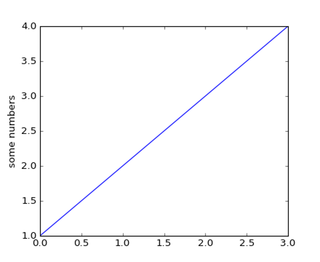
You may be wondering why the x-axis ranges from 0-3 and the y-axis from 1-4. If you provide a single list or array to the plot() command, matplotlib assumes it is a sequence of y values, and automatically generates the x values for you. Since python ranges start with 0, the default x vector has the same length as y but starts with 0. Hence the x data are [0,1,2,3].
plot() is a versatile command, and will take an arbitrary number of arguments. For example, to plot x versus y, you can issue the command:
plt.plot([1, 2, 3, 4], [1, 4, 9, 16])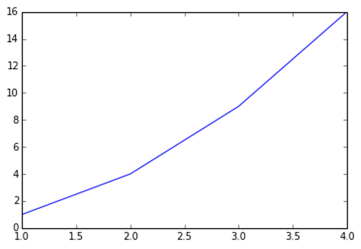
For every x, y pair of arguments, there is an optional third argument which is the format string that indicates the color and line type of the plot. The letters and symbols of the format string are from MATLAB, and you concatenate a color string with a line style string.
The default format string is ‘b-‘, which is a solid blue line. For example, to plot the above with red circles, you would Issue:
import matplotlib.pyplot as plt

plt.plot([1,2,3,4], [1,4,9,16], 'ro')
plt.axis([0, 6, 0, 20])

plt.show()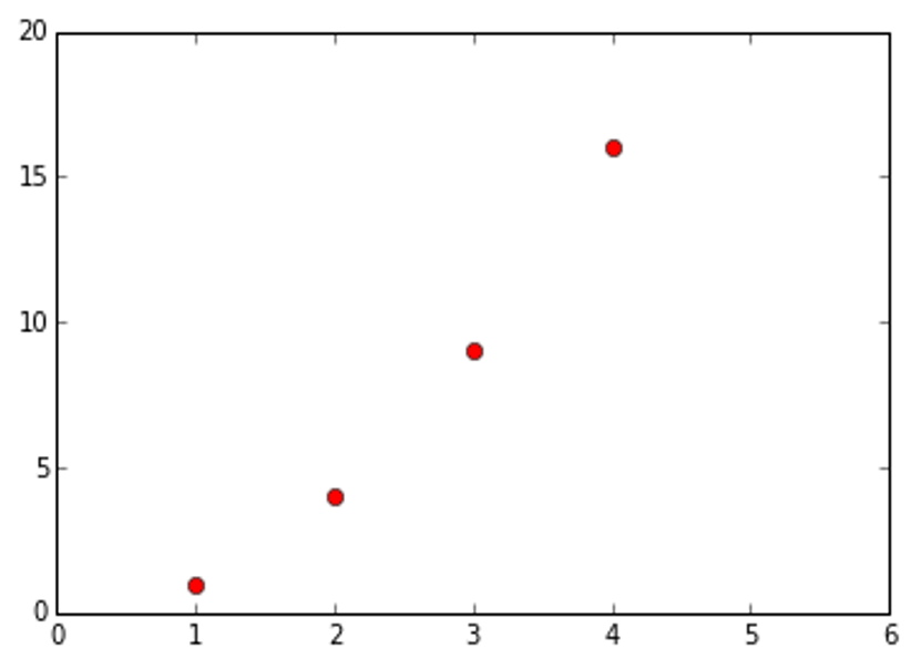
If matplotlib were limited to working with lists, it would be fairly useless for numeric processing. Generally, you will use numpy arrays. In fact, all sequences are converted to numpy arrays internally. The example below illustrates a plotting several lines with different format styles in one command using arrays:
import numpy as np
import matplotlib.pyplot as plt

# evenly sampled time at 200ms intervals
t = np.arange(0., 5., 0.2)

# red dashes, blue squares and green triangles
plt.plot(t, t, 'r--', t, t**2, 'bs', t, t**3, 'g^')

plt.show()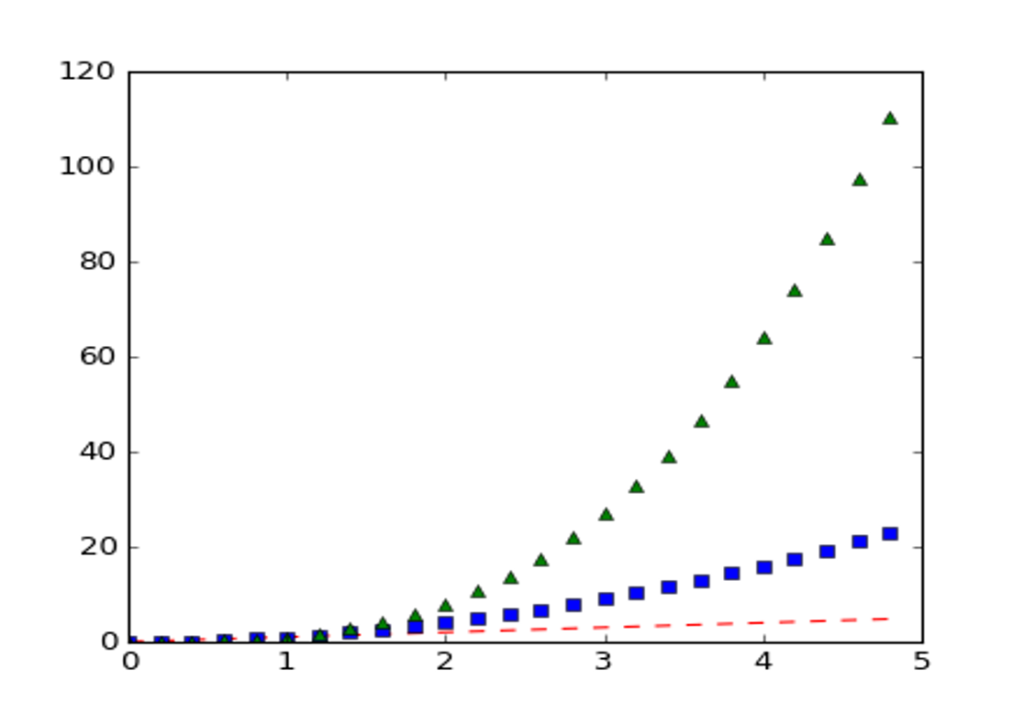
Working with text
The text() command can be used to add text in an arbitrary location, and the xlabel(), ylabel() and title() are used to add text in the indicated locations.
import numpy as np
import matplotlib.pyplot as plt

mu, sigma = 100, 15

x = mu + sigma * np.random.randn(10000)

n, bins, patches = plt.hist(x, 50, normed=1, facecolor='g', alpha=0.75)

plt.xlabel('Smarts')
plt.ylabel('Probability')
plt.title('Histogram of IQ')
plt.text(60, .025, r'$\mu=100,\ \sigma=15$')
plt.axis([40, 160, 0, 0.03])
plt.grid(True)
plt.show()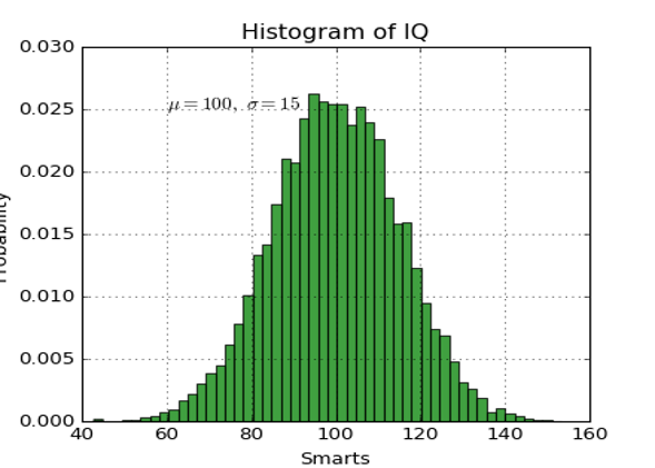
Visit Documentation for more: http://matplotlib.org/index.html
Seaborn
Seaborn is a Python visualization library built on top of matplotlib. It provides a high-level interface for drawing attractive and informative statistical graphics. It works seamlessly with pandas DataFrames—a big plus when working with biological datasets.
Usually, you will have your data in Pandas DataFrame, you’ll plot your main plot using Seaborn, and then annotate it with Matplotlib. Also, there are options to directly use Seaborn without Matplotlib.
import seaborn as sns
import pandas as pd
import matplotlib.pyplot as plt
Bar Plot: Compare Categories
# Simulated gene expression dataset
data = pd.DataFrame({
    'Gene': ['GeneA']*3 + ['GeneB']*3,
    'Tissue': ['Liver', 'Brain', 'Heart']*2,
    'Expression': [12.1, 9.3, 7.8, 15.2, 11.0, 10.5]
})

sns.barplot(data=data, x='Tissue', y='Expression', hue='Gene')
plt.title("Gene Expression across Tissues")
plt.show()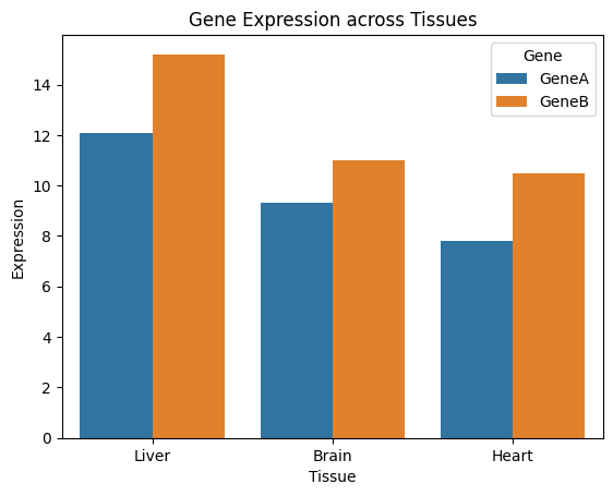
Line Plot — Trends Over Time
data = pd.DataFrame({
    'Time': list(range(0, 10)) * 2,
    'Population': [10, 25, 40, 70, 90, 110, 130, 145, 155, 160,
                   10, 20, 35, 60, 85, 100, 120, 135, 140, 145],
    'Medium': ['LB']*10 + ['Minimal']*10
})

sns.lineplot(data=data, x='Time', y='Population', hue='Medium')
plt.title("Bacterial Growth in Two Media")
plt.show()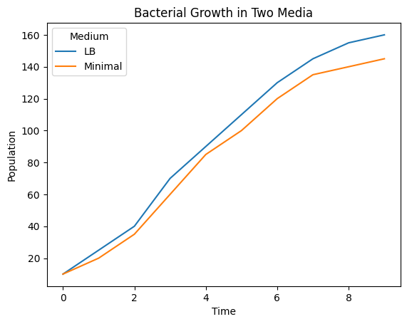
Scatter Plot — Correlation Between Variables
data = pd.DataFrame({
    'GeneA': [10, 12, 15, 18, 25, 30, 28, 24, 22, 20],
    'GeneB': [8, 11, 14, 17, 23, 31, 29, 23, 21, 19],
    'Tissue': ['Liver', 'Liver', 'Brain', 'Brain', 'Heart', 'Heart', 'Liver', 'Brain', 'Heart', 'Liver']
})

sns.scatterplot(data=data, x='GeneA', y='GeneB', hue='Tissue')
plt.title("Co-expression of GeneA and GeneB")
plt.show()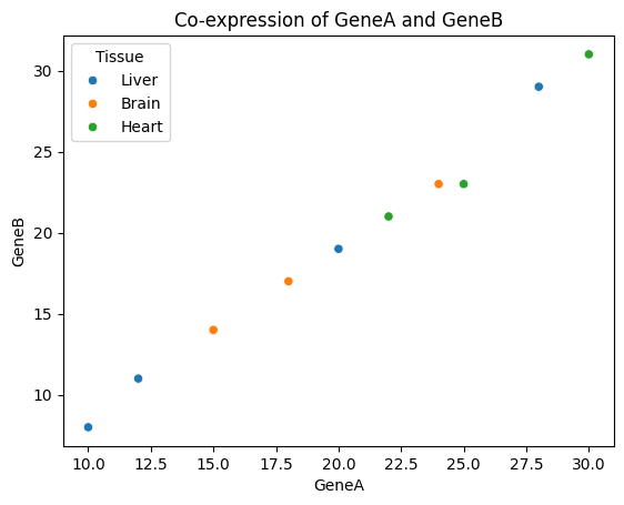
Box Plot — Distribution Summary
data = pd.DataFrame({
    'Tissue': ['Liver']*5 + ['Brain']*5 + ['Heart']*5,
    'Expression': [10, 12, 13, 14, 11, 8, 9, 7, 8.5, 10, 14, 15, 13, 12.5, 14.5]
})

sns.boxplot(data=data, x='Tissue', y='Expression')
plt.title("Distribution of Expression Levels")
plt.show()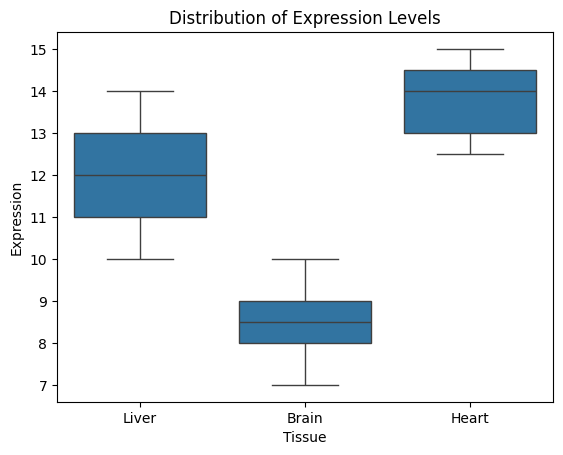
Violin Plot — Distribution + Density
sns.violinplot(data=data, x='Tissue', y='Expression')
plt.title("Violin Plot of Expression per Tissue")
plt.show()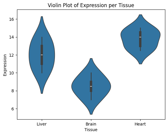
Pair Plot — Pairwise Relationships
import seaborn as sns
import pandas as pd
import matplotlib.pyplot as plt
import numpy as np

df = pd.DataFrame({
    'GeneA': np.random.normal(10, 2, 50),
    'GeneB': np.random.normal(15, 3, 50),
    'GeneC': np.random.normal(12, 4, 50),
    'Condition': ['Healthy']*25 + ['Diseased']*25
})

sns.pairplot(df, hue='Condition')
plt.suptitle("Pairwise Gene Co-expression", y=1.02)
plt.show()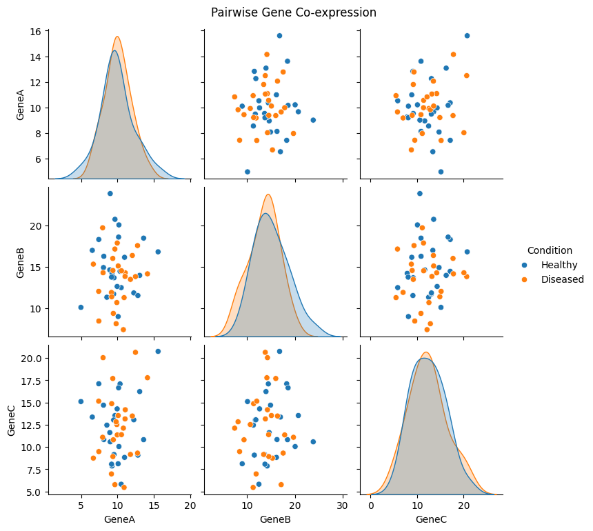
Tips for Biological Data
- Clean your data with
pandas(.dropna(),.groupby(),.melt()) before plotting. - Use
hue,style, andsizein Seaborn to add layers of metadata (e.g., sample type, treatment). - For large data, consider downsampling or summarizing to reduce clutter.
- Combine Seaborn with
matplotlibto tweak plot appearance.
Seaborn example with a simulated dataset
Part 1: Simulated GEO Expression Dataset
import pandas as pd
import numpy as np
import seaborn as sns
import matplotlib.pyplot as plt
sns.set(style="whitegrid")
# Simulate metadata for 30 samples
np.random.seed(42)
samples = [f"Sample_{i}" for i in range(1, 31)]
conditions = ['Control']*15 + ['Treated']*15
metadata = pd.DataFrame({'SampleID': samples, 'Condition': conditions})
# Simulate expression data for 3 genes
expression_data = pd.DataFrame({
'SampleID': samples,
'GeneA': np.random.normal(loc=10, scale=2, size=30),
'GeneB': np.random.normal(loc=15, scale=2.5, size=30),
'GeneC': np.random.normal(loc=12, scale=1.5, size=30)
})
# Merge metadata and expression data
df_expr = pd.merge(metadata, expression_data, on='SampleID')
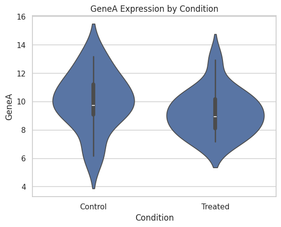
# 1. Violin Plot for GeneA Expression
plt.figure()
sns.violinplot(data=df_expr, x='Condition', y='GeneA')
plt.title("GeneA Expression by Condition")
plt.show()
# 2. Line Plot - Circadian Expression Simulation
timepoints = np.tile(np.arange(0, 24, 4), 2)
geneX_expr = np.sin(np.pi * timepoints / 12) * 5 + 10 + np.random.normal(0, 0.5, len(timepoints))
df_time = pd.DataFrame({
    'Time': timepoints,
    'Expression': geneX_expr,
    'Condition': ['Control']*6 + ['Treated']*6
})

plt.figure()
sns.lineplot(data=df_time, x='Time', y='Expression', hue='Condition', marker='o')
plt.title("GeneX Circadian Expression")
plt.show()
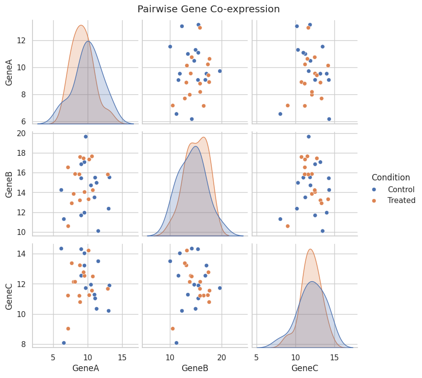
# 3. Pairplot of Gene Co-expression
sns.pairplot(df_expr[['GeneA', 'GeneB', 'GeneC', 'Condition']], hue='Condition')
plt.suptitle("Pairwise Gene Co-expression", y=1.02)
plt.show()
Part 2: Simulated SNP Dataset
samples = [f"Sample_{i}" for i in range(1, 21)]
chromosomes = ['Chr1', 'Chr2', 'Chr3', 'Chr4', 'Chr5']
# Simulate SNP counts
np.random.seed(1)
snp_data = pd.DataFrame({
'SampleID': np.repeat(samples, len(chromosomes)),
'Chromosome': chromosomes * len(samples),
'SNP_Count': np.random.poisson(lam=50, size=len(samples)*len(chromosomes))
})
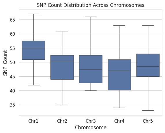
# 4. Box Plot of SNP Count Distribution
plt.figure()
sns.boxplot(data=snp_data, x='Chromosome', y='SNP_Count')
plt.title("SNP Count Distribution Across Chromosomes")
plt.show()
# 5. Bar Plot of Average SNPs per Chromosome
avg_snp = snp_data.groupby('Chromosome')['SNP_Count'].mean().reset_index()

plt.figure()
sns.barplot(data=avg_snp, x='Chromosome', y='SNP_Count')
plt.title("Average SNP Count per Chromosome")
plt.show()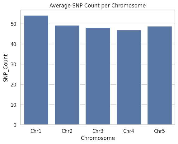
# 6. Heatmap of SNPs per Sample/Chromosome
pivot_table = snp_data.pivot(index='SampleID', columns='Chromosome', values='SNP_Count')

plt.figure(figsize=(10, 8))
sns.heatmap(pivot_table, cmap='Blues', annot=True)
plt.title("SNP Counts per Sample and Chromosome")
plt.show()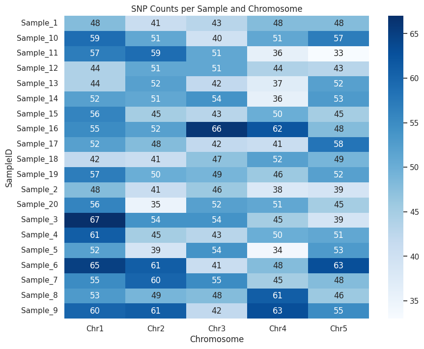
Don’t forget to check out documentation for Seaborn: https://seaborn.pydata.org/examples/index.html
Go to the index of Py4Bio.
Leave a Reply