

This is the Chapter 8 of Py4Bio.
What is NumPy?
NumPy is an acronym for “Numeric Python”
Open source extension module for Python
Provides fast precompiled functions for mathematical and numerical routines.
Powerful data structures for efficient computation of multi-dimensional arrays and matrices.
The module supplies a large library of high-level mathematical functions to operate on these matrices and arrays.
Comparison between core python and numpy
When we say “Core Python”, we mean Python without any special modules, i.e. especially without NumPy.
The advantages of Core Python:
– high-level number objects: integers, floating point
-containers: lists with cheap insertion and append methods, dictionaries with fast lookup
Advantages of using Numpy with Python:
– array oriented computing
– efficiently implemented multi-dimensional arrays
– designed for scientific computation
NumPy is the foundation of the Python scientific stack.
A simple numpy example
Before we can use NumPy we will have to import it. It has to be imported like any other module:
>>> import numpyBut you will hardly ever see this. Numpy is usually renamed to np:
>>> import numpy as npWe have a list with values, e.g. temperatures in Celsius. We will turn this into a one-dimensional numpy array:
>>> cvalues = [25.3, 24.8, 26.9, 23.9]
>>> C = np.array(cvalues)
>>> print(C)
Let’s assume, we want to turn the values into degrees Fahrenheit. This is very easy to accomplish with a numpy array. The solution to our problem can be achieved by simple scalar multiplication:
>>> print(C * 9 / 5 + 32)Compared to this, the solution for our Python list is extremely awkward:
>>> fvalues = []
>>> for i in cvalues:
...		fvalues.append(i*9/5 + 32)
...
>>> print(fvalues)
Creation of evenly spaced values
There are functions provided by Numpy to create evenly spaced values within a given interval.
One uses a given distance ‘arange’ and the other one ‘linspace’ needs the number of elements and creates the distance automatically.
Arange
The syntax of arange:
arange([start,] stop[, step,], dtype=None)arange returns evenly spaced values within a given interval. The values are generated within the half-open interval ‘[start, stop)’ If the function is used with integers, it is nearly equivalent to the Python built-in function range, but arange returns an ndarray rather than a list iterator as range does.
If the ‘start’ parameter is not given, it will be set to 0. The end of the interval is determined by the parameter ‘stop’.
Usually, the interval will not include this value, except in some cases where ‘step’ is not an integer and floating pointround-off affects the length of output ndarray. The spacing between two adjacent values of the output array is set with the optional parameter ‘step’.
The default value for ‘step’ is 1. If the parameter ‘step’ is given, the ‘start’ parameter cannot be optional, i.e. it has tobe given as well. The type of the output array can be specified with the parameter ‘dtype’. If it is not given, the type will be automatically inferred from the other input arguments.
>>> import numpy as np
>>> a = np.arange(1, 10)
>>> print(a)

>>> # compare to range:
>>> x = range(1,10)
>>> print(x)
>>> # x is an iterator
>>> print(x)

>>> # some more arange examples:
>>> x = np.arange(10.4)
>>> print(x)
>>> x = np.arange(0.5, 10.4, 0.8)
>>> print(x)
>>> x = np.arange(0.5, 10.4, 0.8, int)
>>> print(x)
Linspace
The syntax of linspace:
linspace(start, stop, num=50, endpoint=True, retstep=False)linspace returns an nd-array, consisting of ‘num’ equally spaced samples in the closed interval [start, stop] or the half-open interval [start, stop). If a closed or a half-open interval will be returned, depends on whether ‘endpoint’ is True or False. The parameter ‘start’ defines the start value of the sequence which will be created.
‘stop’ will the end value of the sequence, unless ‘endpoint’ is set to False. In the latter case, the resulting sequence will consist of all but the last of ‘num + 1’ evenly spaced samples. This means that ‘stop’ is excluded.
Note that the step size changes when ‘endpoint’ is False. The number of samples to be generated can be set with ‘num’, which defaults to 50. If the optional parameter ‘endpoint’ is set to True (the default), ‘stop’ will be the last sample of the sequence. Otherwise, it is not included.
>>> import numpy as np

>>> # 50 values between 1 and 10:
>>> print(np.linspace(1, 10))

>>> # 7 values between 1 and 10:
>>> print(np.linspace(1, 10, 7))

>>> # excluding the endpoint:
>>> print(np.linspace(1, 10, 7, endpoint=False))
We haven’t discussed one interesting parameter so far. If the optional parameter ‘retstep’ is set, the function will also return the value of the spacing between adjacent values. So, the function will return a tuple (‘samples’,’step’):
>>> import numpy as np

>>> samples, spacing = np.linspace(1, 10, retstep=True)
>>> print(spacing)

>>> samples, spacing = np.linspace(1, 10, 20, endpoint=True, retstep=True)
>>> print(spacing)

>>> samples, spacing = np.linspace(1, 10, 20, endpoint=False, retstep=True)
>>> print(spacing)
Time Comparison Between Python Lists and NumPy Arrays
import time

size_of_vec = 1000

def pure_python_version():
	t1 = time.time()
	X = range(size_of_vec)
	Y = range(size_of_vec)
	Z = []
	for i in range(len(X)):
		Z.append(X[i] + Y[i])
	return time.time() - t1


def numpy_version():
	t1 = time.time()
	X = np.arange(size_of_vec)
	Y = np.arange(size_of_vec)
	Z = X + Y
	return time.time() - t1


t1 = pure_python_version()
t2 = numpy_version()

print(t1, t2)

print("Numpy is in this example " + str(t1/t2) + " faster!")
Creating arrays: Zero-dimensional arrays
It’s possible to create multidimensional arrays in numpy. Scalars are zero dimensional. In the following example, we will create the scalar 42. Applying the ndim method to our scalar, we get the dimension of the array. We can also see that the type is a “numpy.ndarray” type.
x = np.array(42)
print(type(x))
print(np.ndim(x))
The above code will return the following result:
<class 'numpy.ndarray'>
0
Creating arrays: One-dimensional arrays
We have already encountered a 1-dimenional array – better known to some as vectors – in our initial example. What we have not mentioned so far, but what you may have assumed, is the fact that numpy arrays are containers of items of the same type, e.g. only integers. The homogenous type of the array can be determined with the attribute “dtype”, as we can learn from the following example:
F = np.array([1, 1, 2, 3, 5, 8, 13, 21])
V = np.array([3.4, 6.9, 99.8, 12.8])

print(F.dtype)
print(V.dtype)
print(np.ndim(F))
print(np.ndim(V))
Creating arrays: Two- and multi-dimensional arrays
Of course, arrays of NumPy are not limited to one dimension. They are of arbitrary dimension. We create them by passing nested lists (or tuples) to the array method of numpy.
A = np.array([	[3.4, 8.7, 9.9],
		[1.1, -7.8, -0.7],
		[4.1, 12.3, 4.8]])

print(A)
print(A.ndim)

B = np.array([	[[111, 112], [121, 122]],
		[[211, 212], [221, 222]],
		[[311, 312], [321, 322]] ])

print(B)
print(B.ndim)
Numpy array shapes are tuples that contains the shape for each dimensions.
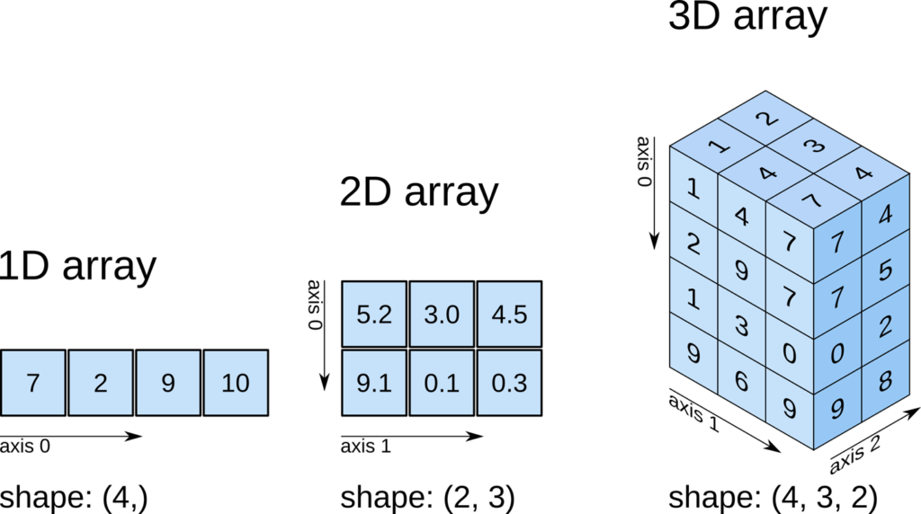
Shape of an array
The function “shape” returns the shape of an array. The shape is a tuple of integers. These numbers denote the lengths of the corresponding array dimension. In other words: The “shape” of an array is a tuple with the number of elements per axis (dimension). In our example, the shape is equal to (6, 3), i.e. we have 6 lines and 3 columns.
x = np.array([ 	[67, 63, 87],
		[77, 69, 59],
		[85, 87, 99],
		[79, 72, 71],
		[63, 89, 93],
		[68, 92, 78]])

print(np.shape(x))

# There is also an equivalent array property:
print(x.shape)
The shape of an array tells us also something about the order in which the indices are processed, i.e. first rows, then columns and after that the further Dimensions.
“shape” can also be used to change the shape of an array.
x.shape = (3, 6)
print(x)
You might have guessed by now that the new shape must correspond to the number of elements of the array, i.e. the total size of the new array must be the same as the old one. We will raise an exception, if this is not the case:
x.shape = (4, 4)Indexing
Assigning to and accessing the elements of an array is similar to other sequential data types of Python, i.e. lists and tuples. We have also many options to indexing, which makes indexing in Numpy very powerful and similar to core Python. Single indexing is the way, you will most probably expect it:
F = np.array([1, 1, 2, 3, 5, 8, 13, 21])

# print the first element of F, i.e. the element with the index 0

print(F[0])

# print the last element of F
print(F[-1])

# Indexing multi-dimensional arrays

A = np.array([	[3.4, 8.7, 9.9],
		[1.1, -7.8, -0.7],
		[4.1, 12.3, 4.8]])

print(A[1][0])

B = np.array([ 	[[111, 112], [121, 122]],						[[211, 212], [221, 222]],
[[311, 312], [321, 322]] ])

print(B[0][1][0])
Slicing
Slicing in an arrya is similar to slicing of lists and tuples. The syntax is the same in numpy for one-dimensional arrays, but it can be applied to multiple dimensions as well.
The general syntax for a one-dimensional array A looks like this:
A[start:stop:step]We illustrate the operating principle of “slicing” with some examples. We start with the easiest case, i.e. the slicing of a one-dimensional array:
S = np.array([0, 1, 2, 3, 4, 5, 6, 7, 8, 9])

print(S[2:5])
print(S[:4])
print(S[6:])
print(S[:])
We will illustrate the multidimensional slicing in the following examples. The ranges for each dimension are separated by commas:
A = np.array([[11,12,13,14,15],
  [21,22,23,24,25],
  [31,32,33,34,35],
  [41,42,43,44,45],
  [51,52,53,54,55]])

print(A[:3,2:])

print(A[3:,:])

printA([:,4:])
Arrays of ones and zeros
There are two ways of initializing Arrays with Zeros or Ones. The method ones(t) takes a tuple t with the shape of the array and fills the array accordingly with ones. By default it will be filled with Ones of type float.
If you need integer Ones, you have to set the optional parameter dtype to int:
import numpy as np

E = np.ones((2,3))
print(E)

F = np.ones((3,4),dtype=int)
print(F)
What we have said about the method ones() is valid for the method zeros() analogously, as we can see in the following example:
Z = np.zeros((2,4))
print(Z)
Exercises
1. Create an arbitrary one dimensional array called “v”.
2. Create a new array which consists of the odd indices of previously created array “v”.
3. Create a new array in backwards ordering from v.
4. What will be the output of the following code:
a = np.array([1, 2, 3, 4, 5])
b = a[1:4]
print(a[1])
5. Create a two dimensional array called “m”.
6. Create a new array from m, in which the elements of each row are in reverse order.
7. Another one, where the rows are in reverse order.
8. Create an array from m, where columns and rows are in reverse order.
9. Slice off the first and last row and the first and last column.
Go to the index of Py4Bio.
Leave a Reply