Microbial pan-genome analysis

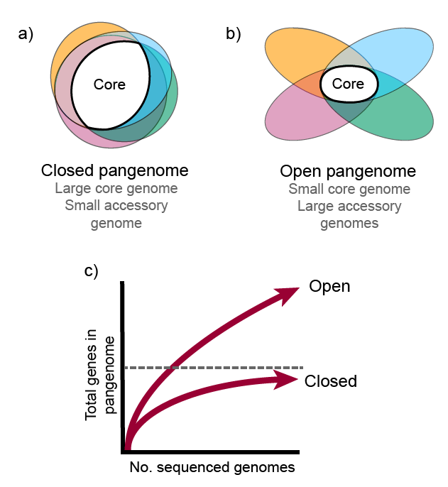
Pan-genome means collection of ALL genome for a particular species. This is a fairly common analysis in microbial genomics.

Compared to eukaryotic organisms, bacterial genomes a fluid. Take randomly two genomes from a bacterial species, chances are that there will be huge genetic differences in terms of gene content. That’s because, conjugation, recombination and horizontal gene transfer (HGT) is very common in bacteria.

Why is so? It is energetically costly to replicate and maintain an extra gene which is not needed for survival. Therefore bacterial genomes tend to carefully curate a set of genes which is absolutely needed in the particular ecological niche it thrives on.

Usually, we can categorize the pan-genome content in three groups: core, accessory, and singleton. The set of genes shared all or most of the member of a species is called core gene. Accessory genes (aka shell) are shared some members, and often these are specific to particular niche adaptation. Finally, all microbial genome tends to contain set of unique genes only observed in an individual member, but not in others. These are called singleton (aka cloud).

How to do pan-genome analysis? Well, you need to gather all available genomes for a species. You may have sequenced some, and downloaded all available genomes from NCBI or any other public databases. Then, you need to do genome annotation and ortholog clustering of all genes. Ortholog clustering will give you a big gene presence-absence table for all genomes, which can be used to get pan-genome statistics.

In this tutorial, we’ll use a set of 44 genomes of Propionibacterium freudenreichii isolates coming from yogurt samples. This has been annotated and ortholog clustering has been done in a previous tutorial.

Technically, this is NOT a pan-genome analysis since we are not using all available genomes from Propionibacterium freudenreichii, rather a small enough dataset for quickly execute the tutorial.

PIRATE will produce a PIRATE.gene_families.ordered.originalIDs.tsv file in the output directory, which we will use as input in R.

You can download the file from here.

Analyze pan-genome using R

library(data.table)
library(dplyr)
library(ggplot2)
library(doParallel)
library(ggpubr)

# Load the ortholog cluster presence absence table as a R data frame
PIRATE.gene_families <- as.data.frame(fread("PIRATE.gene_families.ordered.originalIDs.tsv"))

# Make a number_genomes column in the data frame
PIRATE.gene_families$number_genomes <- 0 

# Update the number of genome where the gene orgholog group was observed
PIRATE.gene_families$number_genomes <- rowSums( !(PIRATE.gene_families[ , 23:length(colnames(PIRATE.gene_families))] == "") )

PIRATE.gene_families <- PIRATE.gene_families[ which(PIRATE.gene_families$number_genomes > 0), ]

head(PIRATE.gene_families)

# Distribution of genes across the strains
gene_total <- colSums( !(PIRATE.gene_families[ , 23:length(colnames(PIRATE.gene_families))] == ""))

gene_total contains total genes per genome. We have some gene content variation in this dataset:

> summary(as.vector(gene_total))   
Min. 1st Qu.  Median    Mean 3rd Qu.    Max.    
2147    2208    2244    2241    2274    2359 

> sd(gene_total)
[1] 43.23223

Let’s plot a histogram:

hist(gene_total)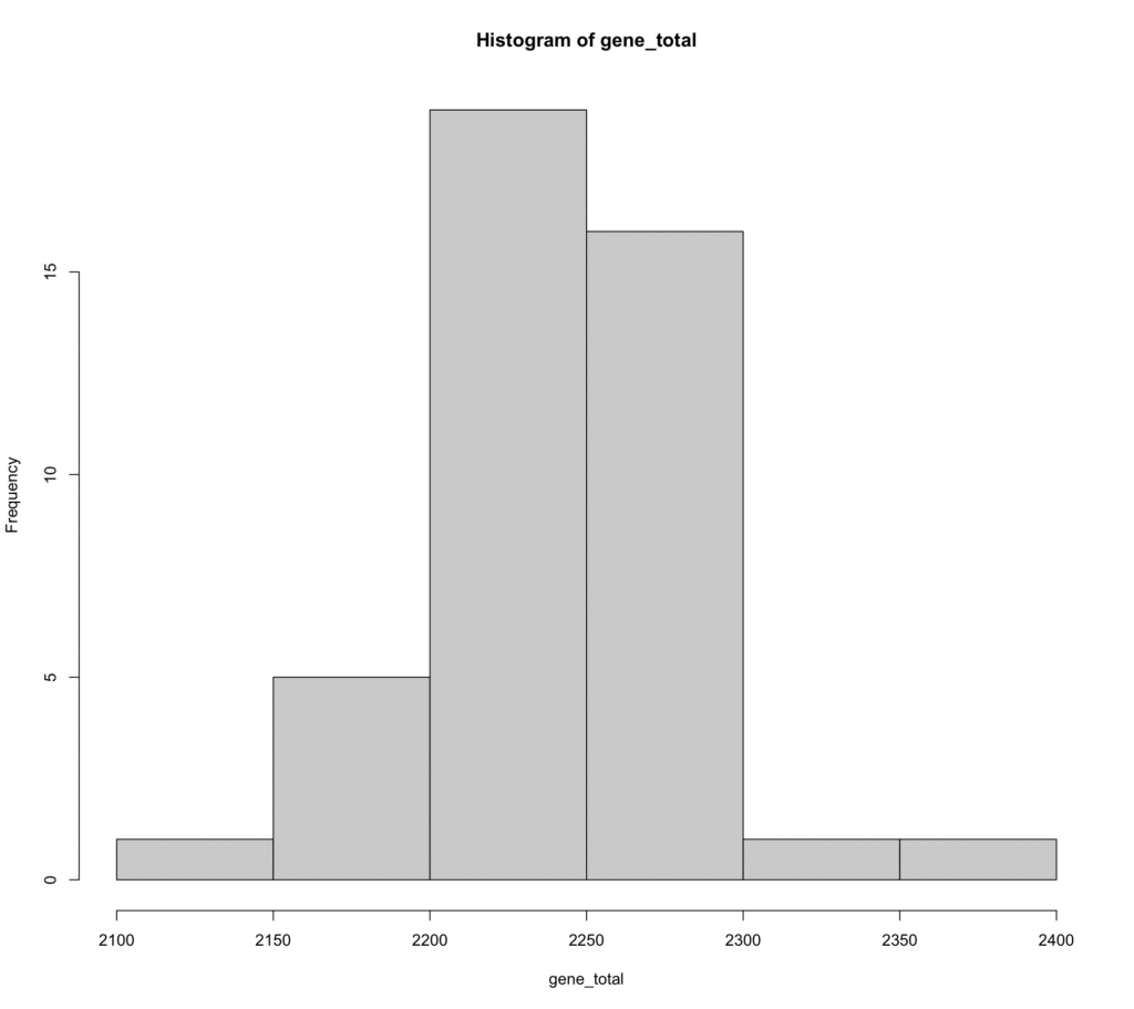

We can get some other interesting pan-genome stats.

# how many gene families are there?
n_gene_fams<-  nrow(PIRATE.gene_families)
n_gene_fans
#3752

The PIRATE gene presence-absence table contains some columns thats not needed in further analysis. We can get rid of those:

# names of cols to exclude
cols_to_exclude <- c("allele_name", "gene_family", "consensus_gene_name", "consensus_product", "threshold", "alleles_at_maximum_threshold", "number_genomes", "average_dose", "min_dose", "max_dose", "genomes_containing_fissions", "genomes_containing_duplications", "number_fission_loci",                    "number_duplicated_loci", "no_loci", "products",                    "gene_names", "min_length(bp)", "max_length(bp)",                    "average_length(bp)", "cluster", "cluster_order")

strains_only <- PIRATE.gene_families[,!names(PIRATE.gene_families) %in% cols_to_exclude]strain_names <- names(strains_only)

Check total genome number present in the dataset:

# Number of genomes
ngenomes <- length(unique(strain_names)) 
ngenomes
43

Let’s get the number of core, accessory, and singletone genes:

# how many of the gene families are in every genome (of 43)
n_gene_fams_core_all <- sum(PIRATE.gene_families$number_genomes == ngenomes)
n_gene_fams_core_all
# 1718 

#how many of the gene families are in every genome (of 43)
n_gene_fams_core_all <- sum(PIRATE.gene_families$number_genomes == ngenomes)
n_gene_fams_core_all
#1718

# that's what percent out of the total?
> (n_gene_fams_core_all*100)/n_gene_fams
# 45.78891

# present in 95% of genomes (n >=248)
cutoff <- round(.95* ngenomes)
 n_gene_fams_core_w95per <- sum(PIRATE.gene_families$number_genomes >= cutoff)
n_gene_fams_core_w95per
# 1913

# that's what percent out of the total?
(n_gene_fams_core_w95per*100)/n_gene_fams
# 50.98614

# how many of the gene families are singletons (accessory)
n_gene_fams_singletons <- sum(PIRATE.gene_families$number_genomes == 1)
n_gene_fams_singletons
# 604

# that's what percent out of the total?
(n_gene_fams_singletons*100)/n_gene_fams
# 16.09808


# how many accessory?)
n_accessory <- n_gene_fams - (n_gene_fams_singletons + n_gene_fams_core_w95per)
n_accessory
# 1235

# that's what percent out of the total?
(n_accessory*100)/n_gene_fams[1] 32.91578

# get accessory average per genome 
n_accessory / ngenomes
#28.72093

We can visualize these stats in a nice plot and report:

# Visualize the distribution of gene presence in a gene family (distribution of core to accessory genes)

# Prepare dataframe for plotting
gene_fam_totals <-as.data.frame(PIRATE.gene_families$number_genomes)

colnames(gene_fam_totals) <- 'count'

# Categorize gene groups
gene_fam_totals$group = 0

for (i in 1:nrow(gene_fam_totals)){  
    if (gene_fam_totals$count[i] == 1) {
               gene_fam_totals$group[i] = "Singleton"  
    } else if (gene_fam_totals$count[i] >= .95*ngenomes){
        gene_fam_totals$group[i] = "Core"  
    } else {
        gene_fam_totals$group[i] = "Accessory"  
    }
}

p1 <- gene_fam_totals %>%  ggplot(aes(x = count)) +  
                geom_bar(aes(fill = group), position = "identity") +  
                ggtitle("Pangenome Distribution by gene ortholog group") +  
                ylab("n gene families") + 
                xlab("n genomes in family") +  
                theme_classic() +  
                theme(plot.title = element_text(size=15), legend.title = element_blank(), legend.position = c(0.85, 0.85)) +  
                scale_fill_manual(name = "", values = c("blueviolet", "coral",  "darkcyan")) +          
                theme_minimal()

p1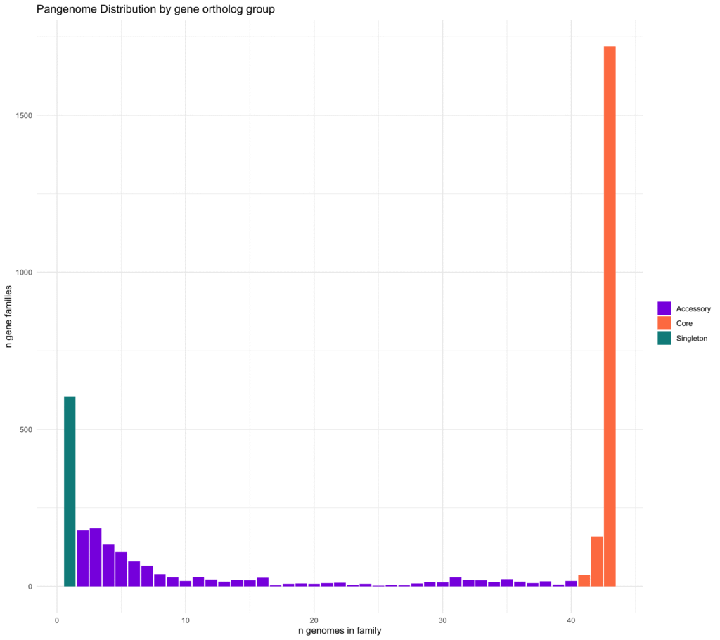

This is a classic U-shaped graph for bacterial pan-genome distribution! In the x-axis, it shows number of genomes, and y-axis is the count of genes present in that number of genomes. The right, orange color bars are core genes, present in almost all genomes. The left green-bar is the singletones. Intermediate purple color bars are the accessory genes.

We can visualize this in doughnut graph.

# Compute percentages
fam_dist_df$fraction <- fam_dist_df$count / sum(fam_dist_df$count)

 Compute the cumulative percentages (top of each rectangle)
fam_dist_df$ymax <- cumsum(fam_dist_df$fraction)

# Compute the bottom of each rectangle
fam_dist_df$ymin <- c(0, head(fam_dist_df$ymax, n=-1))

# Compute label position
fam_dist_df$labelPosition <- (fam_dist_df$ymax + fam_dist_df$ymin) / 2

# Compute a good labelfam_dist_df$label <- paste0(fam_dist_df$category, "\n", fam_dist_df$count)

# Plot
p2 <- ggplot(fam_dist_df, aes(ymax=ymax, ymin=ymin, xmax=4, xmin=3, fill=category)) +  
        geom_rect() +  
        geom_text( x=1.5, aes(y=labelPosition, label=label, color=category), size=4) + 
        # x here controls label position (inner / outer)  
        scale_fill_manual(values=c("blueviolet", "coral",  "darkcyan")) +  
        scale_color_manual(values=c("blueviolet", "coral",  "darkcyan")) +  
        coord_polar(theta="y") +  xlim(c(-1, 4)) +  theme_void() +
        theme(legend.position = "none")

p2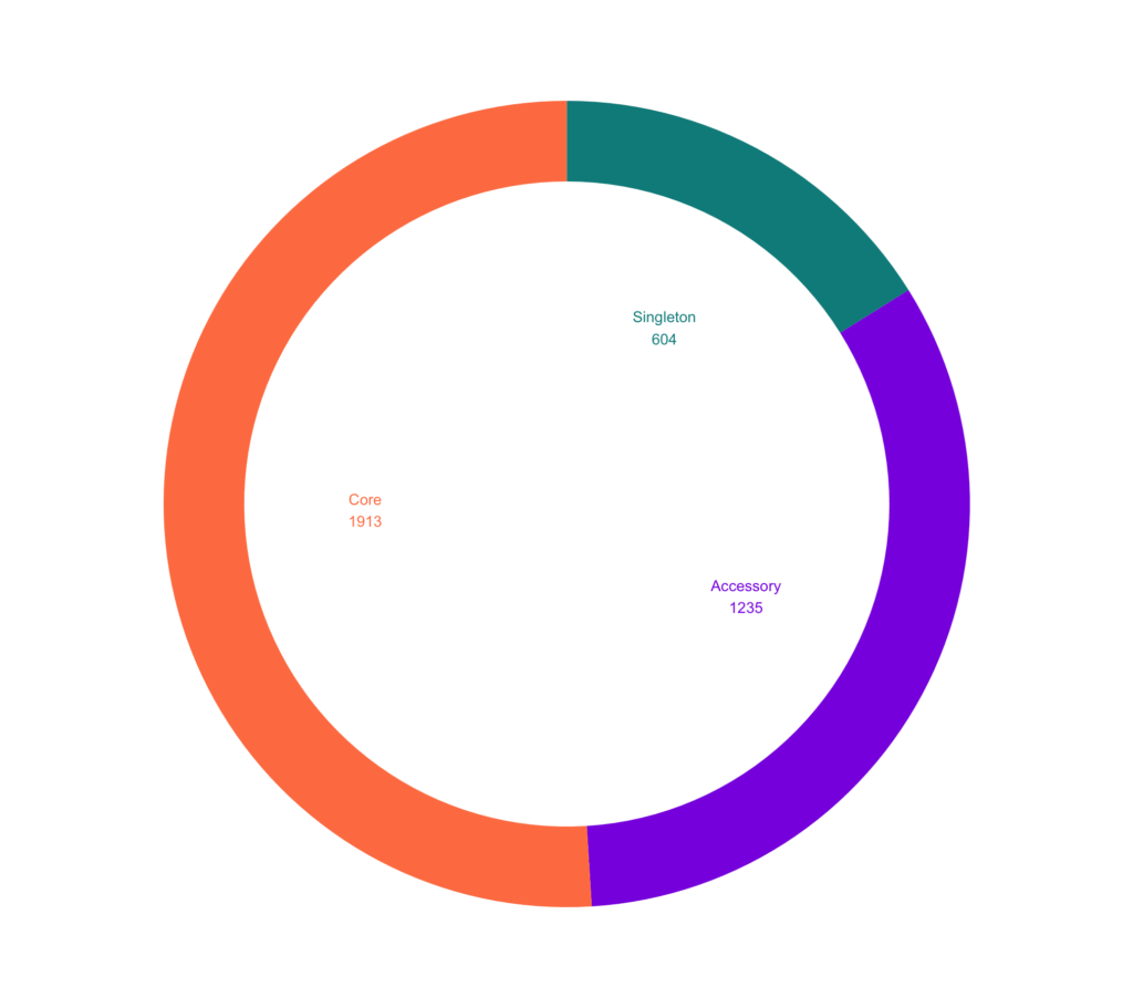

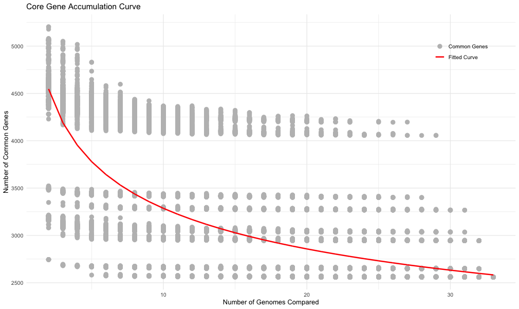
Make a gene accumulation curve

What is a gene accumulation curve?

binary_df <- strains_only %>%   mutate_all(~ as.numeric(nzchar(.)))

count_all_ones <- function(df) {  
        num_cols <- ncol(df)  
        count_cases <- df %>%    
                filter(rowSums(.) == num_cols) %>%                                    
                nrow()  
        return(count_cases)}

find_common_genes <- function(df, cols) {  
        common_genes <- count_all_ones(df[cols])
        return(common_genes)}


# Initialize dataframe to store results
results <- data.frame(  NumGenomes = integer(),  CommonGenes = integer(),  TotalGenes = integer())

# Initialize an empty list to store results
result_list <- list()

# Setup parallel backend to use many processorscores=detectCores()
cl <- makeCluster(cores[1]-2) #not to overload your computer

registerDoParallel(cl) 

# Generate combinations and count common genes
# Initialize an empty list to store results

for(num_genomes in 2:ncol(binary_df)) {  
         rand_combs <- replicate(1000, sample(names(binary_df), num_genomes), simplify = FALSE)
        print(num_genomes)  
        
        local_results <- foreach(i = 1:length(rand_combs), .combine = rbind, .packages = 'dplyr') %dopar% {    
                common_genes_count <- find_common_genes(binary_df, rand_combs[[i]])    
                tota_genes_count <- sum(rowSums(binary_df[rand_combs[[i]]]) > 0)    
                data.frame(NumGenomes = num_genomes, CommonGenes = common_genes_count, TotalGenes = tota_genes_count)  }  
result_list[[num_genomes - 1]] <- local_results  # Store results in list
}

# Stop the parallel backend
stopCluster(cl)

# Combine all results into one data frame
results <- do.call(rbind, result_list)


# Fit power law

# Log-transform the data
results <- results %>%   
       mutate(log_NumGenomes = log(NumGenomes), log_CommonGenes = log(CommonGenes), log_TotalGenes = log(TotalGenes))

head(results)

# Fit a linear model to the log-transformed datalm_model_common <- lm(log_CommonGenes ~ log_NumGenomes, data = results)
lm_model_all <- lm(log_TotalGenes ~ log_NumGenomes, data = results)

# Get the coefficients
coefficients_common <- coef(lm_model_common)
intercept_common <- coefficients_common[1]
slope_common <- coefficients_common[2]

coefficients_all <- coef(lm_model_all)
intercept_all <- coefficients_all[1]
slope_all <- coefficients_all[2]

# Create a data frame for the fitted power law curvefitted_curve <- results %>%  
       mutate(FittedCommonGenes = exp(intercept_common) * NumGenomes^slope_common)


# Core genome size based on accumulation curveexp(intercept_common) * max(results$NumGenomes)^slope_common

fitted_curve <- fitted_curve %>%  
       mutate(FittedAllGenes = exp(intercept_all) * NumGenomes^slope_all)

p3 <- ggplot(results, aes(x = NumGenomes, y = CommonGenes)) +  
       geom_point(aes(color = "Common Genes"), size = 3) +  
       geom_line(data = fitted_curve, aes(x = NumGenomes, y = FittedCommonGenes, color = "Fitted Curve"), size = 1) +  
       scale_color_manual(name = "",                     values = c("Common Genes" = "grey", "Fitted Curve" = "red")) +  
       labs(title = "Core Gene Accumulation Curve",       x = "Number of Genomes Compared",       y = "Number of Common Genes") +  
       theme_minimal() +  
       theme(legend.position = c(0.95, 0.95),  legend.justification = c("right", "top"))


p3

p4 <- ggplot(results, aes(x = NumGenomes, y = TotalGenes)) +  
        geom_point(aes(color = "Total Genes"), size = 3) +  
        geom_line(data = fitted_curve, aes(x = NumGenomes, y = FittedAllGenes, color = "Fitted Curve"), size = 1) +  
        scale_color_manual(name = "",                     values = c("Total Genes" = "grey", "Fitted Curve" = "red")) +  
        labs(title = "Pan Genome Accumulation Curve",       x = "Number of Genomes Compared",       y = "Number of Total Genes") +  
        theme_minimal() +  
        theme(legend.position = c(0.95, 0.05), legend.justification = c("right", "bottom"))

Is the pan-genome open or closed?