
Category: Data Visualization
-

Microbial pan-genome analysis
Pan-genome means collection of ALL genome for a particular species. This is a fairly common analysis in microbial genomics. Compared to eukaryotic organisms, bacterial genomes a fluid. Take randomly two genomes from a bacterial species, chances are that there will be huge genetic differences in terms of gene content. That’s because, conjugation, recombination and horizontal…
-

Annotation of Bacterial Genomes
This is Part 5 of tutorial series: NGS Workflow for Genome Assembly to Annotation for Hybrid Bacterial Data We’ll be use hybrid sequencing data (Illumina and Nanopore). This tutorial has five parts. Disclaimer: This post is a work in progress. This is genome assembly and annotation workflow that I use for microbial genomics. Previously, I used…
-

Creating a Publication Quality Phylogeny Using ggtree
A decade ago, circa 2012-2013, I used MEGA5 to infer phylogeny using simple Neighbour-Joining methods, and used the figure generated by MEGA5 to present and publish my results. Later, when I started learning other phylogeny reconstruction methods like Maximum Likelihood (ML) and Bayesian (which does not draw the tree for you), I started to explore…
-

A tool to visualize fastq alignment with quality-score
Do you need to eyeball through fastq alignment file, with special features to highlight the quality score of each bases? Introducing fastqviz, a Streamlit app which can do just that. I made it quite some time ago to visualize some amplicon data for my own project. You can upload your fastq file. The fastqviz viewer…
-

Quick PCA analysis from sequence alignment data in R
Sometimes you need to visualize SNP data from a small Fasta file. PCA analysis is a great way to look for any distribution pattern.
-
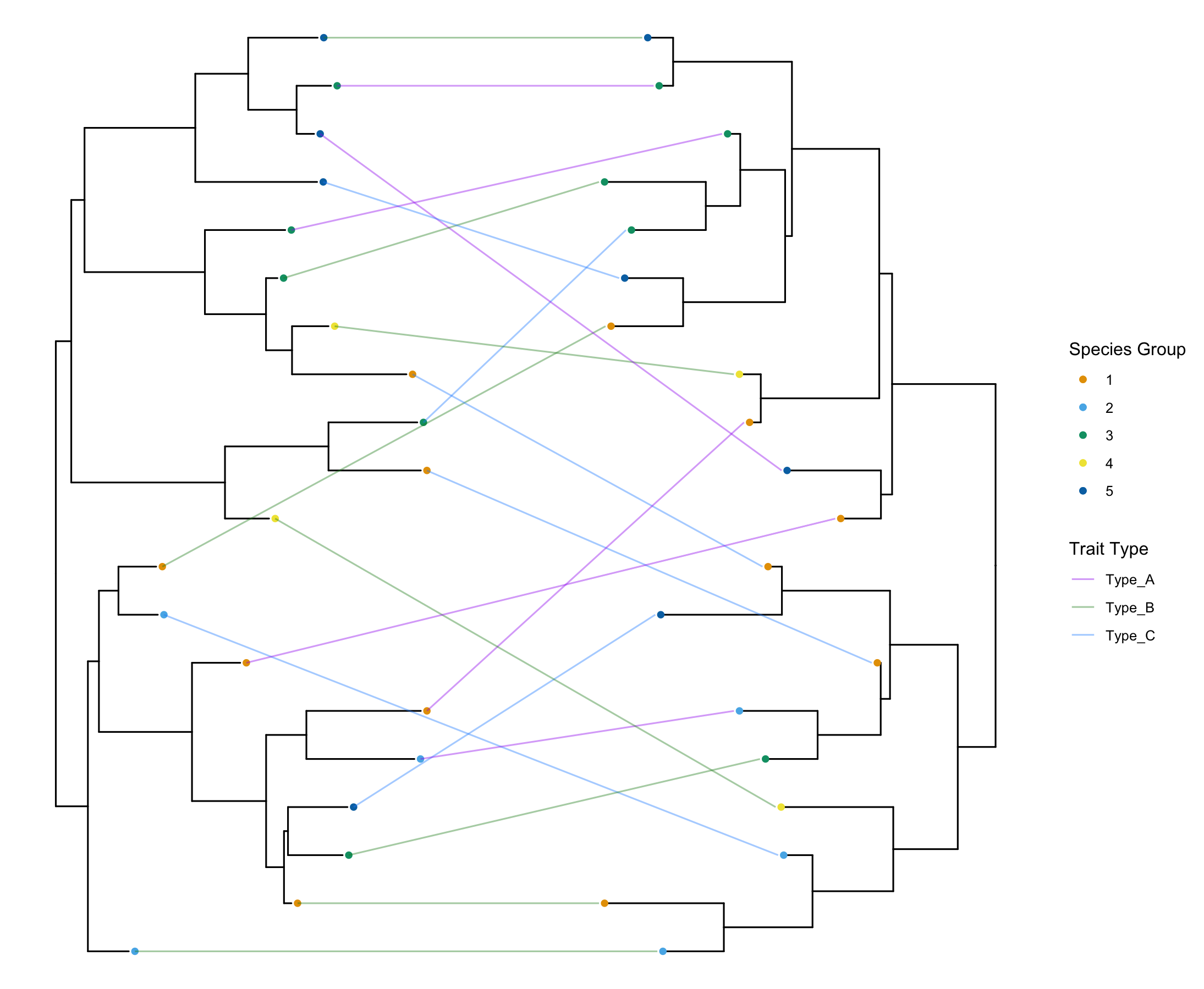
How to make Co-phylogeny plot: easy tanglegram in R (Updated Method)
Tanglegrams are co-phylogeny which is a very powerful visualization tool to examine co-evolution. Here is a tutorial on how to make them in R.