Quick PCA analysis from sequence alignment data in R

It’s common to do principal component analysis (PCA) for large SNP data in VCF format. However, sometimes you want to do a simpler analysis for a very small dataset. Let’s say, you have a gene alignment (or a supermatrix alignment of several genes) and want to visualize SNP structures in the sequence alignment file using PCA. In this post, I’ll show you how to do just that.

library("adegenet")
library("ggplot2")

snp <- fasta2genlight('~/path/to/fasta', snpOnly=T)
meta <- read.table('~/path/to/meta', sep=',', header = T)

fasta2genlight is a nice function from the Adgenet library that extract SNPs from alignment. It also detect the ploidy of your dataset, but do not forget to check the poidy by `snp$ploidy`.

We load our sequence alignment file with this function, and we also load a meta file that contains sequence features that we are interested to visualize in the PCA. The meta file must have a column containing isolate ids that matched fasta id as well. The meta file may look like the following:

Strain	SamplingSite	Species
Isolate1	Site X	A
Isolate2	Site Y	B
…	…	…

Now, we match isolate ids from meta using Strain column and ind.names from genlight object that contains our SNPs. And we also visualize the SNP distribution in the alignment as well.

snp$pop = as.factor(meta[match(snp$ind.names, meta$Strain),]$SamplingSite)

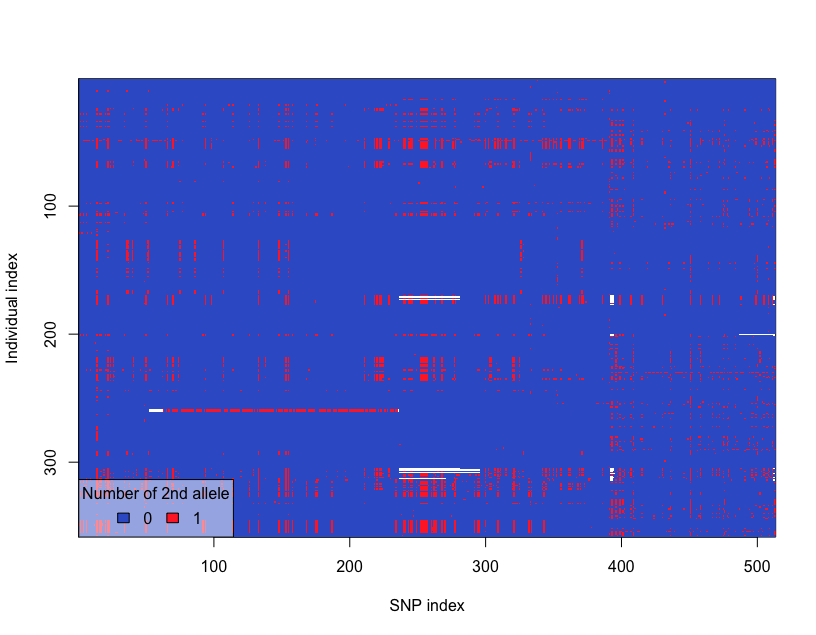
# Heat map of genotype
glPlot(snp)

The SNP distribution heatmap looks like following:

Let’s create the PCA object from SNP data and visualize the Igenvalues for each principal component:

# PCA
pca <- glPca(snp, nf=10)

barplot(100*pca$eig/sum(pca$eig), main="Eigenvalues", col=heat.colors(length(pca$eig)))

# fast plot
scatter(pca, psi='bottomright')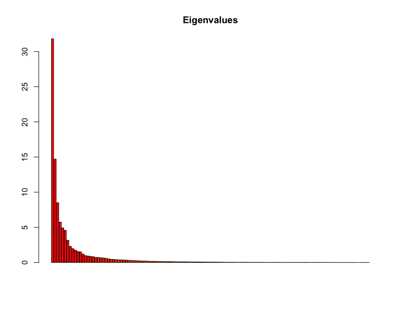

Based on the above plot, we may decide which components we want to visualize. The scatter plot generated by the previous code block is quick but messy. Therefore we decide to play with ggplot.

pca.dataset = as.data.frame(pca$scores)
pca.dataset$isolates = rownames(pca.dataset)
pca.dataset$pop = as.factor(meta[match(snp$ind.names, meta$Strain),]$SamplingSite)
pca.dataset$spp = as.factor(meta[match(snp$ind.names, meta$Strain),]$Species)

ggplot(pca.dataset, aes(PC1, PC2, fill=spp)) + geom_point(shape=21, size=3, alpha=0.7)
ggplot(pca.dataset, aes(PC1, PC3, fill=spp)) + geom_point(shape=21, size=3, alpha=0.7)

Here, we are building a new dataset based on the PCA scores. We also attach two features from the metafile that we intend to visualize. Finally, we draw any two principal components and use the fill variable to select the feature we like to visualize (here we are using spp). The final plot looks like the following:

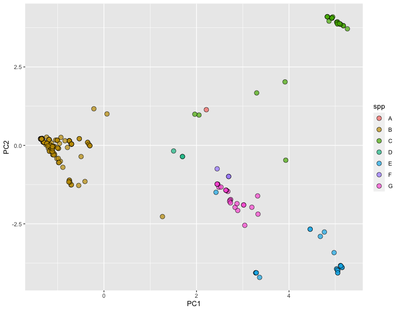
We are definitely seeing some clustering by species in the SNP data!