Creating a Publication Quality Phylogeny Using ggtree

A decade ago, circa 2012-2013, I used MEGA5 to infer phylogeny using simple Neighbour-Joining methods, and used the figure generated by MEGA5 to present and publish my results. Later, when I started learning other phylogeny reconstruction methods like Maximum Likelihood (ML) and Bayesian (which does not draw the tree for you), I started to explore many other tree software, including FigTree (which is a handy click-and-annotate phylogeny software). ML phylogeny seems to be the minimum requirement for inferring phylogeny, and using MLSA (multi-locus sequence analysis) is even better. However, how do you generate publication quality phylogeny can be a challenge for beginner.

Also, now a days, phylogeny comes with a large set of meta-data, which are different traits associated with the strain/isolate sample, and having a phylogeny that decorates those meta-data and/or traits, enhance the figure a ton. In almost all cases, I use ggtree in R to draw publication quality phylogeny. ggtree is a versatile package which is build up on ggplot, and uses the Grammar of Graphics philosophy.

`ggtree` has an excellent documentation, but sometime a beginner can get lost into the detail. Here, I’m going to show you how to effectively use ggtree.

Dataset Preparation

This tutorial involves a dataset that contains sequences and metadata from the viral hemorrhagic septicemia virus (VHSV). This virus is a fish novirhabdovirus (negative stranded RNA virus) with an unusually broad host spectra: it has been isolated from more than 80 fish species in locations
around the Northern hemisphere. This dataset contains two files. One contains sequences encoding the viral surface glycoprotein of VHSV in fasta format. The other contains key metadata information in comma separated format (csv).

You can download the sequence alignment and the meta data by using this link. It’s a good idea to check the alignment, or repeat the alignment. You can use the following command to align the file.

$ mafft input.fasta > output.fasta.aln

Let’s make a maximum likelihood tree using the sequence alignment file. For that, we’ll use IQTree. In command line, we’ll use the following in the command line (assuming UNIX/Linux-like environment):

$ iqtree2 -s input.fasta.aln -bb 1000 -alrt 1000

This essentially use 1,000 times bootstrapping method to estimate the branch support. It will generate several output files in the working directory, but we are interested with the file that has .treefile extension. This is basically a Newick file containing final tree structure and has following content:

(AU-8-95:0.0110853930,(CH-FI262BFH:0.0131606836,(DK-200098:0.0013234532,DK-9995144:0.0000020037)99.8/100:0.0095448338)5.1/70:0.0007266124,((((((((DK-1p40:0.0019814256,DK-1p86:0.0019791590)75.7/94:0.0006552849,((DK-1p8:0.0000009962,(((((DK-4p37:0.0000009962,SE-SVA14:0.0006552195)86/99:0.0006552116,DK-5e59:0.0013125627)0/71:0.0000009962,SE-SVA-1033:0.0000009962)77.3/94:0.0006575521,((DK-6p403:0.0006554966,SE-SVA31:0.0006552486)0/87:0.0000009962,UK-MLA98-6HE1:0.0000009962)85.6/99:0.0019740842)77.5/93:0.0006543360,KRRV9601:0.0006553725)0/18:0.0000009962)0/30:0.0000009962,UK-9643:0.0033009123)77.8/95:0.0006560440)98.9/100:0.0054037876,DK-M.rhabdo:0.0026551354)96/100:0.0043776662,((((((DK-1p53:0.0006552547,DK-1p55:0.0000009962)100/100:0.0816574081,(US-Makah:0.0285238290,US-Goby1-5:0.0140596973)100/100:0.1210587228)42.7/80:0.0177927800,(((DK-4p101:0.0098251613,((DK-4p168:0.0013122432,(UK-H17-2-95:0.0026479867,(UK-H17-5-93:0.0006596353,UK-MLA98-6PT11:0.0013170177)77.3/99:0.0006373176)76/99:0.0006677116)81/99:0.0010715311,IR-F13.02.97:0.0055701665)86.1/93:0.0020013365)74.8/98:0.0009424015,FR-L59X:0.0128785543)95.4/99:0.0075727445,UK-860-94:0.0158862312)100/100:0.0465186423)99.9/100:0.0335638269,GE-1.2:0.0179781031)90.3/92:0.0051635315,(((DK-2835:0.0040046788,(DK-5123:0.0028521912,DK-5131:0.0044304383)80.7/91:0.0031551868)100/100:0.0132948882,DK-Hededam:0.0099447283)72.3/72:0.0008326513,DK-F1:0.0114591421)0/63:0.0000023809)80.3/84:0.0007470511,((FI-ka422:0.0032962818,FI-ka66:0.0000009962)94.8/99:0.0026330173,NO-A16368G:0.0019938953)92.1/97:0.0020400611)60.6/76:0.0002709980)97.9/97:0.0054269715,(FR-1458:0.0099871942,FR-2375:0.0066707318)90.3/95:0.0027197253)93.8/98:0.0031614425,(((((((((((DK-200027-3:0.0020084658,DK-200079-1:0.0020144602)75.7/95:0.0006214026,(DK-9795568:0.0019708808,DK-9995007:0.0013112285)0/83:0.0000009962)84.7/84:0.0006605296,DK-9895093:0.0013136956)0/73:0.0000009962,DK-7380:0.0026325958)49.8/81:0.0012856327,DK-9595168:0.0020294085)94.9/99:0.0026889998,DK-6045:0.0000009962)97.1/100:0.0026359927,DK-7974:0.0039625622)0/87:0.0000009962,DK-5151:0.0000009962)77.1/96:0.0006719096,DK-6137:0.0006446279)100/100:0.0115821189,((DK-3592B:0.0019722385,(DK-3946:0.0006549746,Fil3:0.0006611759)0/46:0.0000009962)0/90:0.0000677760,DK-3971:0.0025622267)98.7/100:0.0068301387)0/88:0.0002780630,(DK-5741:0.0000009962,(DK-9695377:0.0013141688,(DK-9895024:0.0000009962,DK-9895174:0.0013101914)88.7/98:0.0013128147)90/99:0.0013135378)99.7/100:0.0082038754)96.8/77:0.0050912618)77.5/64:0.0033956556,FR-0284:0.0121745715)77.8/91:0.0028167185,FR-0771:0.0001499888)98.7/100:0.0075098885);

The meta file look like this:

Strain	Host	Water	Country	ACCNo	Year
AU-8-95	Rainbow trout	Fresh water	AU	AY546570.1	1995
CH-FI262BFH	Rainbow trout	Fresh water	CH	AY546571.1	1999
DK-1p40	Rockling	Sea water	DK	AY546575.1	1996
…	…	…	..	…	…

It is important that the first column of the meta file contains the same strain names in the fasta file.

First Inspection

Now that we have our Newick tree file, we can load it in R and visualize it right away. Lets do the following:

library(ggtree) # for plotting tree
library(phangorn) # for midpoint root of tree

vshv.tree <- read.tree('Tree_tutorial/Phylogeny_module_example_data.fasta.aln.treefile')


meta <- read.table('Tree_tutorial/Phylogeny_module_tutorial_meta_data.csv', sep=',', header=T)


vshv.tree <- midpoint(vshv.tree)

What we are doing here, is loading necessary packages (ggtree and phagorn), loading tree and meta data, and mid-point rooting the tree. But there is a problem with the read.tree command. Although it is very varsatile Newick file loader, but phylogeny reconstruction software like IQTree, BEAST often adds other tree-related info on the Newick file, and this command can not parse them very well. So, lets modify the script to use advanced IQTree specific parsing command:

library(ggtree) # for plotting tree
library(phangorn) # for midpoint root of tree
library(treeio) # for loading special tree 




vshv.tree <- read.tree('Tree_tutorial/Phylogeny_module_example_data.fasta.aln.treefile')
meta <- read.table('Tree_tutorial/Phylogeny_module_tutorial_meta_data.csv', sep=',', header=T)
vshv.tree <- midpoint(vshv.tree)


vshv.tree <- read.iqtree('Tree_tutorial/Phylogeny_module_example_data.fasta.aln.treefile')
vshv.tree@phylo <- midpoint(vshv.tree@phylo)

# Just tree
plot(vshv.tree@phylo)

Notice how we are using read.iqtree command now and using the phylo object to specifically midpoint the tree, keeping other tree data coming with IQTree untouched. Finally, plotting it will produce something like this:

This looks mundane, nothing exciting. Let’s start using ggtree specific magics to ornament it.

Demystifying ggtree object

To associate the meta-data, which was loaded as a R data-frame, we use the %<+% sign, which allow us to use different columns of the meta data-frame to ornament different part of the tree. For example:

# Lets add tip point

t1 <- ggtree(vshv.tree) %<+% meta +
  geom_tippoint(aes(color=Host))

This will generate the following phylogeny, where tip-points shows the host associated with the meta.

IQTree Newick file comes with a bootstrap support value (--bb option) which has both SH_aLRT and UFboot values. We want to show branches that has high support for both of these (i.e. ≥ 70). But for that, we need to add an indicator for branches that satisfy both condition.

When we define a ggtree object using t1 <- ggtree(vshv.tree) %<+% meta + geom_tippoint(aes(color=Host)), it attaches the meta info as well as tree-branch and tips info coming from original Newick tree-file in the data placeholder, which we can use by t1$data. So let’s update this to have a new column of a variable that satisfy both bootstrap values by the following:

# Circular layout
t1 <- ggtree(vshv.tree, layout="circular") %<+% meta +
  geom_tippoint(aes(color=Host))


# Add bootstrap support

t1$data$bootstrap <- '0'

t1$data[which(t1$data$SH_aLRT >= 70 & t1$data$UFboot  >= 70),]$bootstrap <- '1'


t1 <- t1 + new_scale_color() +
 
 geom_tree(aes(color=bootstrap == '1')) +
 
 scale_color_manual(name='Bootstrap', values=setNames( c('black', 'grey'), c(T,F)), guide = "none")


t1

Notice that we have given a circular layout to the tree. We’ve initiated a bootstrap column with a value of 0 and updated it to 1 if it satisfy our condition. The tree now look like this:

The tree starts to look beautiful, but wait, we can do more.

Show Metadata in Heat-Map

A great way to show other meta data associated with your phylogeny is to add a heat-map. But we need to have separate color layers for separate data-columns. Also, we need to use a good color-palette. For drawing heat map, we need ggtree library. So before starting, we need to add the following libraries:

library(ggtree) #for heat-map
library(ggnewscale) #for new color/fill scale
library(viridis) #using special color scale

Let’s define the meta-data columns individually so that we can call that for vizualization. We are interested in the Water column, which is categorical variable and Year column, which contain continuous variable.

# Lets add heat-map specific dataframe

meta.water <- as.data.frame(meta[,'Water'])

colnames(meta.water) <- 'Water'
rownames(meta.water) <- meta$Strain


meta.year <- as.data.frame(meta[,'Year'])
colnames(meta.year) <- 'Year'
rownames(meta.year) <- meta$Strain

For each variable, we have prepared a data.frame containing single column, add coumn- and row-names to it. Now let’s draw the phylogeny:

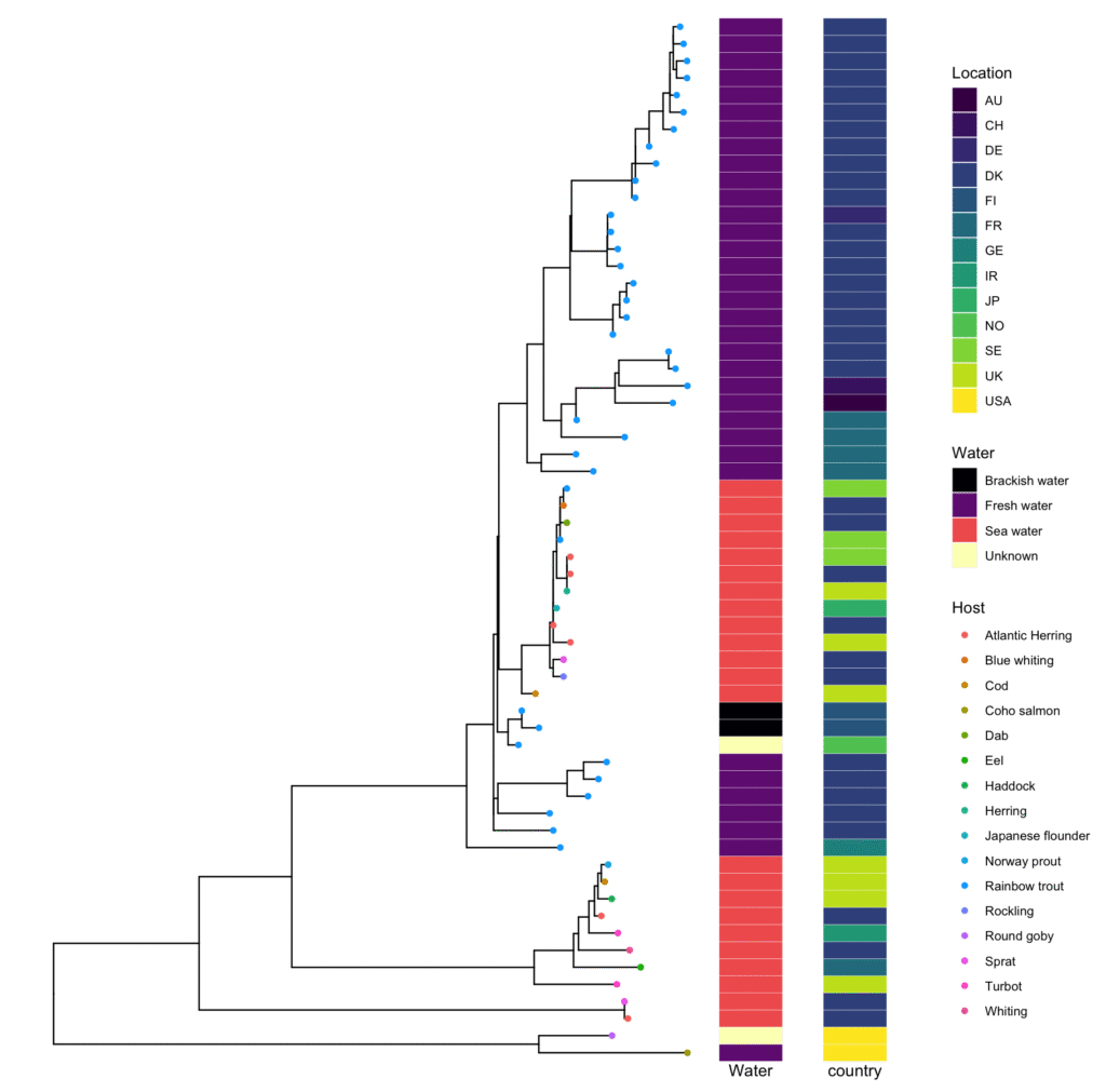
# Categorical variable
t2 <- gheatmap(t1, meta.water, width=0.2) + 
  scale_fill_viridis_d(option="A", name="Country") +
  new_scale_fill()
  


# Continuous variable
t2 <- gheatmap(t2, meta.year, width=0.1, offset=0.05) + 
  scale_fill_viridis(option="D", name="Year")

Notice that we are passing t1 into first gheatmap command and define new tree t2, and passing the t2 again for second gheatmap command. Also, we are defining a new fill scale using new_scale_fill() after the first gheatmap done its drawing, for the second gheatmap to draw upon. And finally, we have two different viridis fill command for categorical vs continuous variable.

Before finally plotting the t2, let’s also add the Country from meta data as tip-label (because why not use all meta-data variable).

# Plot tiplab2

t2 + geom_tiplab2(aes(label=Country), color="gray40", offset=0.003, size=3)

So now, this is the final look:

I hope you liked this tutorial! You can get the full code from my GitHub repo here.

Other Useful Tree Manipulation

Coming up next

• getMRCA
• get_taxa_name
• extract.clade