

For any microbiology project, constructing a phylogenetic tree is an important analysis. A confusing one too — because there are many decisions to make along the way. These decisions can be both technical and hypothesis-driven.
How to Build a Dataset for Phylogeny
Let’s say someone has isolated and sequenced a few microbial strains. The most frequent question I get from beginners is: how do I build the dataset for making a phylogeny? In other words, which bacterial strains should be included in the tree alongside the strain of interest?
This decision depends on the hypothesis being tested or the question being asked. Are we trying to identify the taxonomy of the isolate? Understand an epidemic outbreak? Explore the ecology of a species in a particular region? How many isolates do we have? How similar or diverse are they? Are we also interested in population genetics, ecology, or evolution?
Usually, it’s a good idea to review the relevant literature and see how similar studies have built their phylogenetic datasets.
Although we are usually interested a particular set of microbes in a relatively narrow (closely related taxonomical group), but it is expected that the phylogeny also contains some distant outgroup for rooting purposes.
Sanity Check
Before doing anything else, always check your sequence alignment! Does the multiple sequence alignment (MSA) look okay? Are there visual issues, obvious mismatches, or poorly aligned regions? Sometimes, you’ll need to manually edit the MSA to clean it up.
Dataset Types
Usually, four types of datasets are used in a conventional phylogenetic tree.
- Single marker (gene tree)
- MLSA (Multi-Locus Sequence Analysis)
- Core genome
- SNP
Using multiple genes is usually better. You can align them separately, concatenate the alignments, and then build a tree. This is known as MLSA.
Choice of gene/marker always depends on the question you are asking (hypothesis). For example, if your target is to determining taxonomy, choose gene(s) that can differentiate between species or sub-species level.
For determining the taxonomy, it was conventional to use 16s rRNA (or ITS for fungi) to create a phylogenetic tree. However, in many cases 16s lacks resolution to differentiate closely related species. So, MLSA is powerful in this regard. One key is: different gene may evolve in different rates. So you need to account for that as well. Here’s a tutorial that I wrote for making a MLSA tree.
Core genome tree is definitely going to give you more resolution. Usually, you need to do ortholog clustering analysis in your genome and filter the core genes, i.e. genes present in almost all of the isolate (>95% of the isolates).
If you want to get an even finer scale phylogeny, you can use SNP tree. However, variant calling can be tricky, because SNP calling depends on the reference-genome used. Therefore, SNP calling can be done within a species group, using a particular ANI similarity cutoff (i.e. strains with >95% or >99% similarity).
Model Selection
Many ignores model selection, but it should be properly executed. This is essentially selecting substitution model that best fits your alignment. Why the substitution model selection important? Because, the observed “substitutions” in the MSA are often underestimate of the history.
Let’s do a simple simulation. Take a sequence of 1000 bp, then copy it 1000 times. In each iteration of copying, let’s say one mutation will be randomly introduced. So, after the iteration of copying is done, if you now compare the last (iteration 1000) sequence and first (iteration 0) sequence, you probably would expect there will be 1000 basepair differences. However, since multiple substitutions can “randomly” occur in the same site, you will get much lower differences!
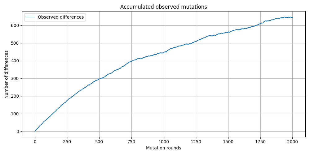
The point is, the observable differences between two sequences are going to be underestimates due to various biological reasons. There are many different substitution models to correct this.
For example, Jukes-Cantor assumes that all possible substitutions are happening in equal frequency. But we know, not all substitutions happens in the same frequency, for example there are more transition mutations compared to transversion. Tamura-Nei model accounts for that.
There are other substitution models like Kimura 2-parametric model, HKY, GTR and different variant of these. How do you know which model to use to correct the substitution counts? There are programs like jModelTests which can analyze your MSA and find the best fit model. Many mainstream phylogenetic reconstruction software can do this automatically. Just be aware of it, and don’t skip this step!
Which tree-building method to use?
I remember, about 10-15 years ago, when I started doing phylogenetic analysis of a RNA-virus (FMDV), doing simple distance based methods (Neighbor-Joining) was the norm. As I read more literature, it became clear that I should start using maximum likelihood and Bayesian techniques.
Yes, distance based methods can reconstruct a phylogeny way faster than any other methods. However, it’s not very reliable in terms of approximating the underlying evolutionary processes. Maximum likelihood methods are accurate, but time consuming. Fortunately, with the invent of multi-core processing, it has now become very much doable in regular personal laptops.
Only tree, or Phylodynamics?
I later started using Bayesian analysis for phylogeny with Beast. Generating Bayesian tree is even more time consuming. However, you can do so much different analysis using beast. Not only you can generate a phylgenetic tree, but you can also estimate mutation rate, create a time-tree, incorporate location info (latitude-longitude), fit epidemiological models and generate many insights which regular phylogenetic tree based method can not analyze.
This field is known as phylodynamics and it provides insights far beyond what standard phylogenetic trees offer.
Bootstrapping confidence
Any tree-building methods are essentially assumptions about the evolutionary history of the isolates. For example, maximum likelihood method tries to fit the data (multiple sequence alignment) with given tree topology, and estimates the probability likelihood. It repeats this over and over again.
Although this is good approximation, however, it still contain weak points. Let’s assume, there are three taxa: A, B, and C. If B closely related to both A and C, the tree may flip between both ((A, B), C) or (A, (B, C)) topology. This can happen specially when there are other evolutionary processes like recombination, horizontal gene transfer happening.
So, in the final tree, how do we test confidence of the branches?
Bootstrapping resamples your alignment many times and rebuilds trees from those resampled datasets. The result: a bootstrap support value for each clade, indicating how often that grouping appears across replicates.
Most phylogenetic tools (e.g., RAxML, IQ-TREE, FastTree) can perform bootstrapping. After that, you should visualize the bootstrap support values to interpret your results properly.
Custom Visualization
No genetic dataset comes alone, it carries a baggage of metadata with it. Visualizing the metadata along with the tree can be highly informative, and help us to formulate new hypothesis. I mainly use the ggtree package in R to visualize the tree with metadata.
Leave a Reply